 |
 |
I frequently encounter the problem of having to find the probability density function (pdf) of some quantity which is a function of several independent random variables with known distributions. For some cases such as addition of two variables, there exists a relatively simple formula (the new pdf is just the convolution of the two) but there is no general magic formula.
Introduction
In a more mathematical language, I need a procedure to find the pdf of a function $y$ where $y : \mathbb{R}^n \rightarrow \mathbb{R}$. If $n=1$ this is quite easy and only involves inverse functions and derivatives. To find an analytical solution in the case where $n>1$, one would generally have to obtain an expression for the cumulative distribution of $y$, and whether it is possible or not to do analytically depends on how complicated the function is.
I wrote a python class that performs this calculation numerically. It is supplied with the function $f(x_1, x_2, x_3, \ldots)$ and the pdfs of $x_1, x_2, x_3, \ldots$ It supplies methods called cdf and pdf which are estimators of what I’m interested in.
The algorithm is quite simple (and perhaps not that efficient). It basically creates a uniform grid in the domain $\mathbb{R}^n$ and maps each gridpoint to its corresponding $y$ and stores for this value what is the joint probability (since all the $x_i$-s are independent, this would just be product of the pdfs). To get the cdf of $y$, I just need to sort these list with respect to $y$ and make a cumulative sum of the probabilities array. I use recursion in the code because it needs a nested loop (to make a multidimensional grid) with an unknown number of levels (depends on the number of variables).
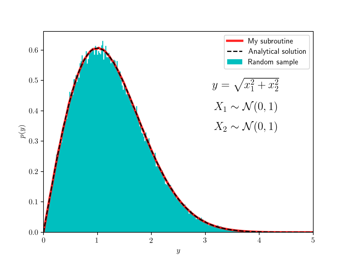
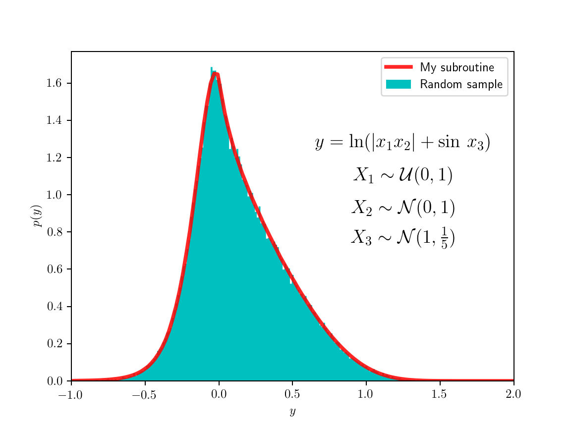
To test the code, I sampled random variables from some known distributions and passed them through various functions, I then made histograms of the image values. The figure on the left shows the simple case where both random variables are normally distributed and the function is the root of the sum of their squares. The resulting distribution can be calculated analytically, it’s related to the Maxwell–Boltzman distribution which is the distribution of three-dimensional vector magnitudes, where each of the component is independently normally distributed (but here I used only two dimensions). The example on the right is a bit crazier (so I didn’t even try to find an analytical solution) and with no actual physical importance. The code for the class is here and the code for the examples is here.
Code
import numpy as np
from scipy.interpolate import interp1d

class probability_of_multivariate_function:
    """
    Probability of a multivariate function.

    Calculates the PDF of `y`, which is some function of multiple random variables: ``y = f(x1, x2, x3, ...)``, given the continuous PDFs of each of its variables and the ranges where these PDFs are to be sampled.

    Parameters
    ----------
    func : callable
        A function of multiple variables f(x1, x2, x3, ...) it should be vectorizable at least on x1 (i.e. return elementwise result when x1 is a numpy vector and all the others are either scalars or vectors of the same length).
    pdfs : list
        A list of callables, each one is the PDF of one of the variables.
    ranges : list
        List of tuples defining the minimum and maximum values for each of the random variables. If the domain of a variable is infinite, one should set the limits such that a very large fraction of the probability distribution is contained between them. #TODO automate this choice.
    points : int or array_like
        The number of samples to take for each variable's distribution. The samples are equally spaced between the given limits. #TODO sample in a smarter way.
    y_min : float
        When constructing the PDF of `y`, values below y=y_min are set to zero.
    y_max : float
        When constructing the PDF of `y`, values above y=y_max are set to zero.
    y_points : int
         When constructing the PDF of `y`, y_points are used. A very large number leads to a noisy result, while a small number leads to inaccuracies.

    Methods
    -------
    cdf
    pdf
    """

    def __init__(self, func, pdfs, ranges, points=512, y_min=None, y_max=None, y_points=256):
        self.n = len(pdfs)
        points = np.array(points)
        if len(points)==1: points.repeat(self.n)
        self.arrays_domain = [np.linspace(ranges[i][0], ranges[i][1], points[i]) for i in range(self.n)]
        self.arrays_image  = [pdfs[i](self.arrays_domain[i]) for i in range(self.n)]
        self.func = func
        self.get_all_combinations()
        i = self.func_result.argsort()
        self.y_values = self.func_result[i] # That's the domain of the new probability space
        self.cdf_values = self.probability[i] # This will be the CDF
        self.cdf_values = np.cumsum(self.cdf_values)
        self.cdf_values /= self.cdf_values[-1]
        # Now attempt to estimate the PDF from the CDF
        self.cdf = interp1d(self.y_values, self.cdf_values)
        if y_min is None: y_min = self.y_values[0]
        if y_max is None: y_max = self.y_values[-1]
        y_new = np.linspace(max(y_min,self.y_values[0]), min(y_max,self.y_values[-1]), y_points)
        c_new = self.cdf(y_new)
        pdf_values = np.diff(c_new)/np.diff(y_new)
        self.pdf = interp1d(0.5*(y_new[1:]+y_new[:-1]), pdf_values, assume_sorted=True, bounds_error=False, fill_value=0)
        del i, self.func_result, self.probability

    def get_all_combinations(self):
        self.j = 0
        self.probability = np.empty(np.prod([len(arr) for arr in self.arrays_domain]))
        self.func_result = np.empty_like(self.probability)
        self.stored_values_domain = np.empty(self.n-1)
        self.stored_values_image  = np.empty(self.n-1)
        self.recursive_part(self.n-1)
        del self.stored_values_domain, self.stored_values_image

    def recursive_part(self, n):
        if n>0:
            for i in range(len(self.arrays_domain[n])):
                self.stored_values_domain[n-1] = self.arrays_domain[n][i]
                self.stored_values_image[n-1]  = self.arrays_image[n][i]
                self.recursive_part(n-1)
        if n==0:
            partial_product = np.prod(self.stored_values_image)
            prod_array = self.arrays_image[0]*partial_product # This is the probability
            self.probability[self.j:self.j+len(self.arrays_domain[0])] = prod_array
            args = [self.stored_values_domain[j] for j in range(self.n-1)]
            args.insert(0, self.arrays_domain[0])
            self.func_result[self.j:self.j+len(self.arrays_domain[0])] = self.func(*args)
            self.j += len(self.arrays_domain[0])
Self criticism
For the method to work and produce a sufficiently smooth pdf, it needs to sample the domain quite well, I found that the results with less than a million points are not so satisfactory. For the example on the left I used 4M points (2048×2048 grid), and for the one on the right used 16M points (256×256×256 grid); though I might have been able to get away with less. A similarly smooth pdf could be obtained just by drawing random samples from the original pdfs and histogramming the results; this way samples don’t have to live in memory at the same time as this experiment can be done in batches (my code could be modified to utilize memory better, in principle). So if there is a reliable random number generator, this Monte Carlo method could be used just as well for this purpose.